Sobol Indices

Sobol’s method is one of the most popular for global sensitivity analysis. It builds on the ANOVA decomposition.

import tntorch as tn
import torch
import time

N = 20
t = tn.rand([32]*N, ranks_tt=10)
t

20D TT tensor:

 32  32  32  32  32  32  32  32  32  32  32  32  32  32  32  32  32  32  32  32
  |   |   |   |   |   |   |   |   |   |   |   |   |   |   |   |   |   |   |   |
 (0) (1) (2) (3) (4) (5) (6) (7) (8) (9) (10)(11)(12)(13)(14)(15)(16)(17)(18)(19)
 / \ / \ / \ / \ / \ / \ / \ / \ / \ / \ / \ / \ / \ / \ / \ / \ / \ / \ / \ / \
1   10  10  10  10  10  10  10  10  10  10  10  10  10  10  10  10  10  10  10  1

With tntorch we can handle all Sobol indices (i.e. for all subsets \(\alpha \subseteq \{0, \dots, N-1\}\)) at once. We can access and aggregate them using the function sobol() and whatever mask is appropriate.

Single Variables

Variance Components

The relative influence (proportion of the overall model variance) attributable to one variable \(n\) only, without interactions with others, is known as its variance component and denoted as \(S_n\). Let’s compute it for the first variable \(x\):

x, y, z = tn.symbols(N)[:3]
start = time.time()
print(tn.sobol(t, mask=tn.only(x)))
print('This compressed tensor has {} parameters; computing this index took only {:g}s'.format(t.numel(), time.time()-start))

tensor(0.1882)
This compressed tensor has 58240 parameters; computing this index took only 0.0380359s

Input parameters \(x, y, \dots\) are assumed independently distributed. By default, uniform marginal distributions are used, but you can specify others with the marginals argument (list of vectors). For instance, if the first variable can take one value only, then its sensitivity indices will be 0 (no matter how strong its effect on the multidimensional model is!):

marginals = [None]*N  # By default, None means uniform
marginals[0] = torch.zeros(t.shape[0])
marginals[0][0] = 1  # This marginal's PMF is all zeros but the first value
tn.sobol(t, tn.only(x), marginals=marginals)

tensor(0.)

Total Sobol Indices

The effect that also includes \(x\)’s interaction with other variables is called total Sobol index (it’s always larger or equal than the corresponding variance component):

tn.sobol(t, x)

tensor(0.2150)

Tuples of variables

What are the indices for the first and third variables \(x\) and \(z\)?

tn.sobol(t, tn.only(x & z))  # Variance component

tensor(0.0005)

tn.sobol(t, x | z)  # Total index

tensor(0.2401)

What’s the relative importance of \(x\) with respect to the group \(\{y, z\}\)?

tn.sobol(t, x & (y|z)) / tn.sobol(t, y|z)

tensor(0.1638)

Closed Sobol Indices

For tuples of variables two additional kinds of indices exist. The closed index aggregates all components for tuples included in \(\alpha\), and for tuple \(\{x, z\}\) it can be computed as follows:

tn.sobol(t, tn.only(x | z))

tensor(0.2100)

Superset Indices

The superset index aggregates all components for tuples that include \(\alpha\):

tn.sobol(t, x & z)

tensor(0.0009)

Counting \(k\)-plets of Variables

We can also easily count the influence of all \(k\)-plets of variables combined:

tn.sobol(t, tn.weight_mask(N, weight=[1]))

tensor(0.9222)

Often, there are different ways to express the same mask. For example, these three are equivalent:

print(tn.sobol(t, x | z))
print(tn.sobol(t, x & ~z) + tn.sobol(t, ~x & z) + tn.sobol(t, x & z))
print(tn.sobol(t, x) + tn.sobol(t, z) - tn.sobol(t, x & z))

tensor(0.2401)
tensor(0.2401)
tensor(0.2401)

The Mean Dimension

Variance components are the basis for an important advanced sensitivity metric, the *mean dimension*. It’s defined as \(D_S := \sum_{\alpha} |\alpha| \cdot S_{\alpha}\) and computed as:

tn.mean_dimension(t)

tensor(1.0831)

We can also compute it in one line by weighting the Sobol indices by their tuple weight (according to the definition of mean dimension):

tn.sobol(t, tn.weight(N))

tensor(1.0831)

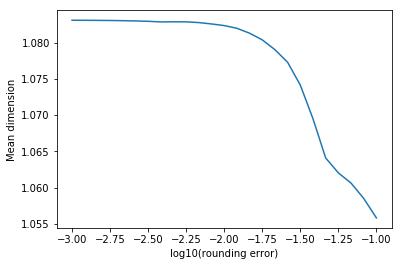
The mean dimension is always greater or equal than 1. It gives a notion of complexity of a multidimensional function (the lower the mean dimension, the simpler it is). For example, rounding a tensor usually results in a lower mean dimension:

import matplotlib.pyplot as plt
%matplotlib inline
import numpy as np

errors = 10**np.linspace(-1, -3, 25)
mean_dimensions = []
for eps in errors:
    mean_dimensions.append(tn.mean_dimension(tn.round(t, eps=eps)))

plt.figure()
plt.plot(np.log10(errors), mean_dimensions)
plt.xlabel('log10(rounding error)')
plt.ylabel('Mean dimension')
plt.show()

We can also compute the restricted mean dimension, i.e. impose certain conditions on the set of tuples that intervene. For example, we can see which of two variables tends to show up more with higher-order terms:

print(tn.mean_dimension(t, mask=x))
print(tn.mean_dimension(t, mask=y))

tensor(1.1355)
tensor(1.3664)

The Dimension Distribution

Last, the *dimension distribution* gathers the relevance of \(k\)-tuples of variables for each \(k = 1, \dots, N\):

start = time.time()
dimdist = tn.dimension_distribution(t)
print(dimdist)
print('Time:', time.time() - start)

tensor([9.2223e-01, 7.2741e-02, 4.7444e-03, 2.6979e-04, 1.3797e-05, 6.4638e-07,
        2.8097e-08, 1.1428e-09, 4.3612e-11, 1.5722e-12, 5.3506e-14, 1.7216e-15,
        5.2287e-17, 1.4966e-18, 4.0144e-20, 1.0023e-21, 2.3034e-23, 4.7723e-25,
        8.6303e-27, 1.3940e-28])
Time: 0.11500120162963867

It can be viewed as a probability mass function, namely the probability of choosing a \(k\)-variable tuple, if tuples are chosen according to their variance components. The expected value of this random variable is the mean dimension. Naturally, the dimension distribution must sum to \(1\):

sum(dimdist)

tensor(1.0000)

Again, we can extract the dimension distribution with respect to any mask:

tn.dimension_distribution(t, mask=y&z)

tensor([0.0000, 0.6815, 0.2870, 0.0293, 0.0021, 0.0001, 0.0000, 0.0000, 0.0000,
        0.0000, 0.0000, 0.0000, 0.0000, 0.0000, 0.0000, 0.0000, 0.0000, 0.0000,
        0.0000, 0.0000])

We just imposed that two variables (\(y\) and \(z\)) appear. Note how, accordingly, the relevance of \(1\)-tuples has become zero since they have all been discarded.