ANOVA Decomposition

The *analysis of variances (ANOVA) decomposition* is well-defined for any square-integrable multidimensional function \(f: \mathbb{R}^N \to \mathbb{R}\). If the input variables \(\{x_0, \dots, x_{N-1}\}\) are independently distributed random variables, the ANOVA decomposition partitions the total variance of the model, \(\mathrm{Var}[f]\), as a sum of variances of orthogonal functions \(\mathrm{Var}[f_{\alpha}]\) for all possible subsets \(\alpha\) of the input variables. Each \(f_{\alpha}\) depends effectively on the variables contained in \(\alpha\) only, and is constant with respect to the rest.

import torch
import tntorch as tn

N = 4
t = tn.rand([32]*N, ranks_tt=5)

Let’s compute all ANOVA terms in one single tensor network:

anova = tn.anova_decomposition(t)
anova

4D TT-Tucker tensor:

 33  33  33  33
  |   |   |   |
 32  32  32  32
 (0) (1) (2) (3)
 / \ / \ / \ / \
1   5   5   5   1

This tensor anova indexes all \(2^N\) functions \(f_{\alpha}\) of the ANOVA decomposition of \(f\), and we can access it using our tensor masks.

Reference: *”Sobol Tensor Trains for Global Sensitivity Analysis”*, R. Ballester-Ripoll, E. G. Paredes, R. Pajarola (2017).

Manipulating the Decomposition

For example, let’s keep all terms that do not interact with \(w\):

x, y, z, w = tn.symbols(N)
anova_cut = tn.mask(anova, ~w)

We can undo the decomposition to obtain a regular tensor again:

t_cut = tn.undo_anova_decomposition(anova_cut)

As expected, our truncated tensor t_cut has become constant with respect to the fourth variable \(w\):

t_cut[0, 0, 0, :].torch()

tensor([6.1559, 6.1559, 6.1559, 6.1559, 6.1559, 6.1559, 6.1559, 6.1559, 6.1559,
        6.1559, 6.1559, 6.1559, 6.1559, 6.1559, 6.1559, 6.1559, 6.1559, 6.1559,
        6.1559, 6.1559, 6.1559, 6.1559, 6.1559, 6.1559, 6.1559, 6.1559, 6.1559,
        6.1559, 6.1559, 6.1559, 6.1559, 6.1559])

How much did we lose by making that variable unimportant?

print('The truncated tensor accounts for {:g}% of the original variance.'.format(tn.var(t_cut) / tn.var(t) * 100))

The truncated tensor accounts for 53.3676% of the original variance.

… which is also what Sobol’s method gives us:

tn.sobol(t, ~w) * 100

tensor(53.3676)

or, equivalently,

tn.sobol(t, tn.only(x | y | z)) * 100

tensor(53.3676)

Note that the empty subfunction \(f_{\emptyset}\) is constant, and its value everywhere coincides with the original function’s mean:

empty = tn.undo_anova_decomposition(tn.mask(anova, tn.none(N)))
print(tn.var(empty))  # It's a constant function
print(empty[0, 0, 0, 0], tn.mean(t))  # Coincides with the global mean

tensor(6.5831e-14)
tensor(8.3357) tensor(8.3357)

Also note that summing all ANOVA subfunctions results in the original function:

all_summed = tn.undo_anova_decomposition(tn.mask(anova, tn.true(N)))
tn.relative_error(t, all_summed)

tensor(1.8894e-08)

Truncating Dimensionality

The low-dimensional terms of the ANOVA decomposition (i.e. terms that depend on a few variables only) are usually the ones that play the most important role in many analytical and real-world models.

We will now approximate our original function as a sum of (at most) bivariate functions. To that end we will use a weight mask tensor.

m = tn.weight_mask(N, [0, 1, 2])  # Keep tuples with zero, one or two '1's
print('We will keep only {:g} of the original ANOVA terms'.format(tn.sum(m)))
t_cut = tn.undo_anova_decomposition(tn.mask(tn.anova_decomposition(t), m))
print('Relative error after truncation: {}'.format(tn.relative_error(t, t_cut)))

We will keep only 11 of the original ANOVA terms
Relative error after truncation: 0.028525682742228935

Visualizing the ANOVA Decomposition

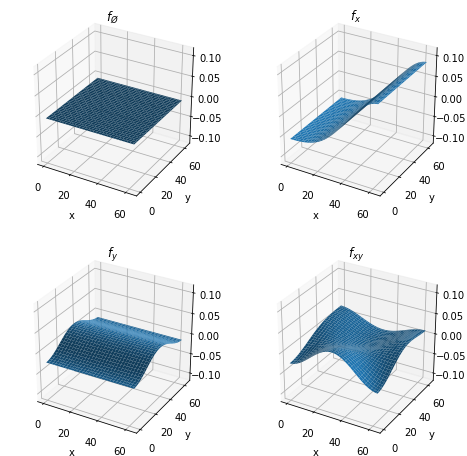
Let’s now restrict ourselves to \(N = 2\) so that we can easily plot the ANOVA subfunctions and get an idea how they look like.

# We set up a smooth 2D tensor, sum of a few cosine wavefunctions
N = 2
t = tn.randn([64]*N, ranks_tt=4, ranks_tucker=3)
t.set_factors('dct')
t

2D TT-Tucker tensor:

 64  64
  |   |
  3   3
 (0) (1)
 / \ / \
1   4   1

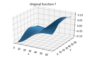
The full function looks like this:

import matplotlib.pyplot as plt
%matplotlib inline
from mpl_toolkits.mplot3d import Axes3D
import numpy as np

fig = plt.figure()
ax = fig.gca(projection='3d')
X, Y = np.meshgrid(np.arange(t.shape[0]), np.arange(t.shape[1]), indexing='ij')
surf = ax.plot_surface(X, Y, t.numpy())
plt.title('Original function $f$')
plt.xlabel('x')
plt.ylabel('y')
plt.show()

Next we will show the \(2^N = 4\) ANOVA subfunctions:

x, y = tn.symbols(N)
anova = tn.anova_decomposition(t)
zlim = [t.numpy().min(), t.numpy().max()]

fig = plt.figure(figsize=(8, 8))

ax = fig.add_subplot(2, 2, 1, projection='3d')
ax.plot_surface(X, Y, tn.undo_anova_decomposition(tn.mask(anova, tn.none(N))).numpy())  # Equivalent to ~x & ~y
plt.xlabel('x')
plt.ylabel('y')
ax.set_zlim3d(zlim[0], zlim[1])
ax.set_title('$f_{\O}$')

ax = fig.add_subplot(2, 2, 2, projection='3d')
ax.plot_surface(X, Y, tn.undo_anova_decomposition(tn.mask(anova, tn.only(x))).numpy())
plt.xlabel('x')
plt.ylabel('y')
ax.set_zlim3d(zlim[0], zlim[1])
ax.set_title('$f_x$')

ax = fig.add_subplot(2, 2, 3, projection='3d')
ax.plot_surface(X, Y, tn.undo_anova_decomposition(tn.mask(anova, tn.only(y))).numpy())
plt.xlabel('x')
plt.ylabel('y')
ax.set_zlim3d(zlim[0], zlim[1])
ax.set_title('$f_y$')

ax = fig.add_subplot(2, 2, 4, projection='3d')
ax.plot_surface(X, Y, tn.undo_anova_decomposition(tn.mask(anova, tn.only(x & y))).numpy())
plt.xlabel('x')
plt.ylabel('y')
ax.set_zlim3d(zlim[0], zlim[1])
ax.set_title('$f_{xy}$')

plt.show()